This is an integrated tutorial about viewscape and dsmSearch. These two packages were initially one before getting published because I thought it would be cool if one can just specify a geographical area without DSM/DEM to compute a viewshed(s). This has been explained the purpose of making the dsmSearch, which was two functions for searching and downloading point cloud data via API.
Of course, viewscape is not designed for just computing the viewshed even if this is the core of the package. A set of function for calculating viewscape metrics (see details) is the main contribution of this package. What’s more, it provides the functionality to subset the viewshed based on the angle and orientation of the field of view and compute the visual magnitude within the viewshed.
Before I start, what is ‘viewshed’ and what is ‘viewscape’ by the way? Basically, I would say viewscape is a concept of analysis relying on viewshed, which is the visible area that can be seen from the location of a observer. Viewscape analysis is to understand the composition of landscape and the structure of viewshed itself and visible objects within the viewshed.
# install packages
install.pakcages("viewscape")
install.pakcages("dsmSearch")
1.Compute viewshed
To compute a viewshed, a viewpoint and a DSM are essential. Let’s download the LiDAR data from a small part of a city. In this tutorial, I take the Central Park (NYC) as an example. First, a bounding box (bbox) is used to locate an area to download the data. lidR, a powerful tool for processing LiDAR data, is used to generate DSM/DEM.
# bbox finder: http://bboxfinder.com/
bbox <- c(-73.976440,40.768793,-73.969628,40.773295)

# download LiDAR (.las)
las <- dsmSearch::get_lidar(bbox = bbox, epsg = 2263)

# constrct DSM and DEM using .las data
dsm <- lidR::rasterize_canopy(las, 5, lidR::dsmtin())
dem <- lidR::rasterize_terrain(las, 5, lidR::tin())
In this case, I just set the center point of the DSM as the viewpoint.
row <- trunc(terra::nrow(dsm)/2)
col <- trunc(terra::ncol(dsm)/2)
cell <- terra::cellFromRowCol(dsm, row, col)
xy <- terra::xyFromCell(dsm, cell)
viewpoint <- c(xy[,1], xy[,2])
# compute viewshed
# the height of the viewpoint is set as 6 feet
viewshed <- viewscape::compute_viewshed(dsm,
                                        viewpoint,
                                        offset_viewpoint = 6)
In real life, we can not see all theoretical visible objects at once with the limited view angle. To present a more realistic viewscape analysis, sector_mask is provided to extract
# subset the viewshed
sub_viewshed <- viewscape::sector_mask(viewshed, c(10,100))
The output ‘viewshed’ object can be written in raster format using visualize_viewshed for further analysis and visualization.
# create a raster of viewshed
viewshed_raster <- viewscape::visualize_viewshed(viewshed, outputtype = "raster")
# plot viewshed overlapping with the DSM
terra::plot(dsm, legend = FALSE)
terra::plot(viewshed_raster, add=TRUE, col = "red")
2. Compute visual magnitude
Binary viewshed only present the locations of visible contents, however, people may be also interested in quantifying the contribution of the visible content in a scene. Therefore, visual magnitude is used to estimate the proportion of each visible area unit within a viewshed. visual_magnitude function implements the visual magnitude algorithm for this purpose.
vm <- viewscape::visual_magnitude(viewshed, dsm)
3. Compute viewscape metrics for multiple viewpoints
Viewscape metrics are meaningful in understanding the experience of urban landscapes, such as perceived restorativeness and visual walkability. I used built-in data of this package to demonstrate whole process of computing viewscape metrics for multiple viewpoints.
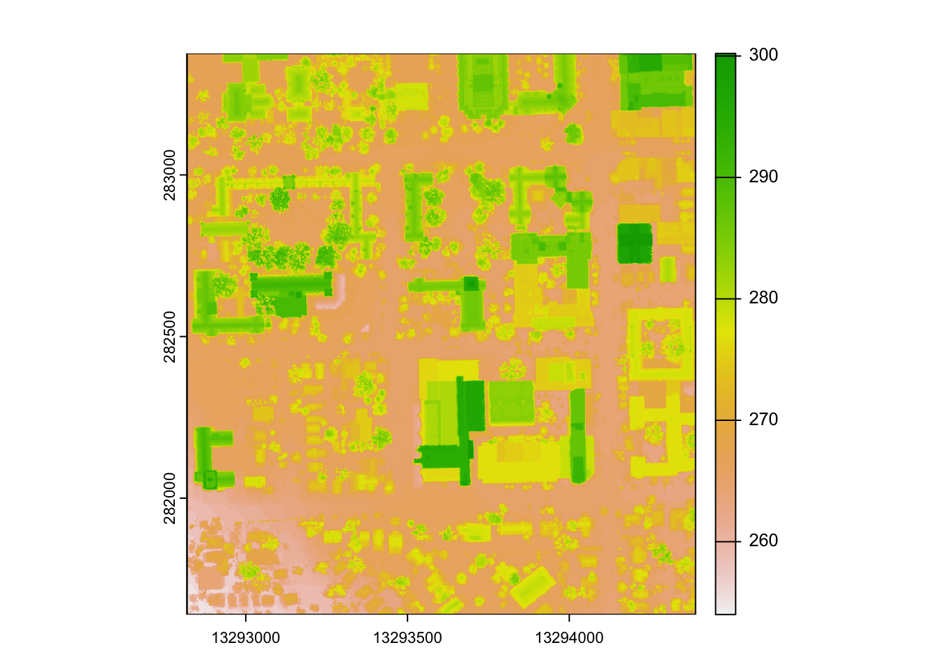
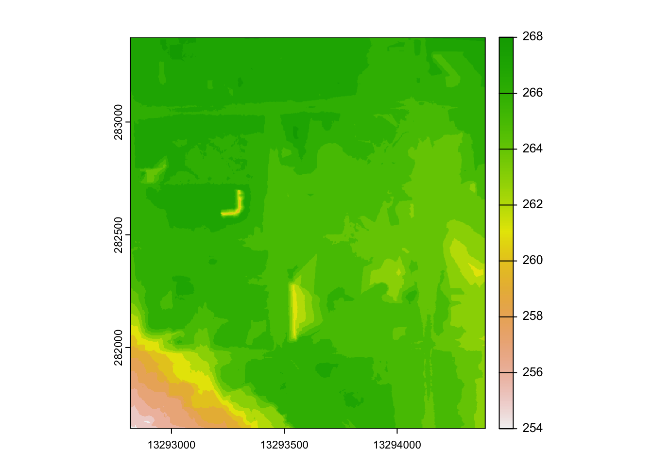
First, I loaded in all data needed for the viewscape analysis. If you don’t have DSM (or DTM), you can use your DTM (or DSM) as DSM (or DTM).
# read a viewpoint
viewpoints <- sf::read_sf(system.file("test_viewpoints.shp",
package = "viewscape"))
# read DSM and DTM
dsm <- terra::rast(system.file("test_dsm.tif",
package ="viewscape"))
dtm <- terra::rast(system.file("test_dtm.tif",
package ="viewscape"))
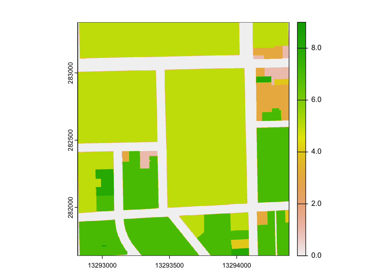
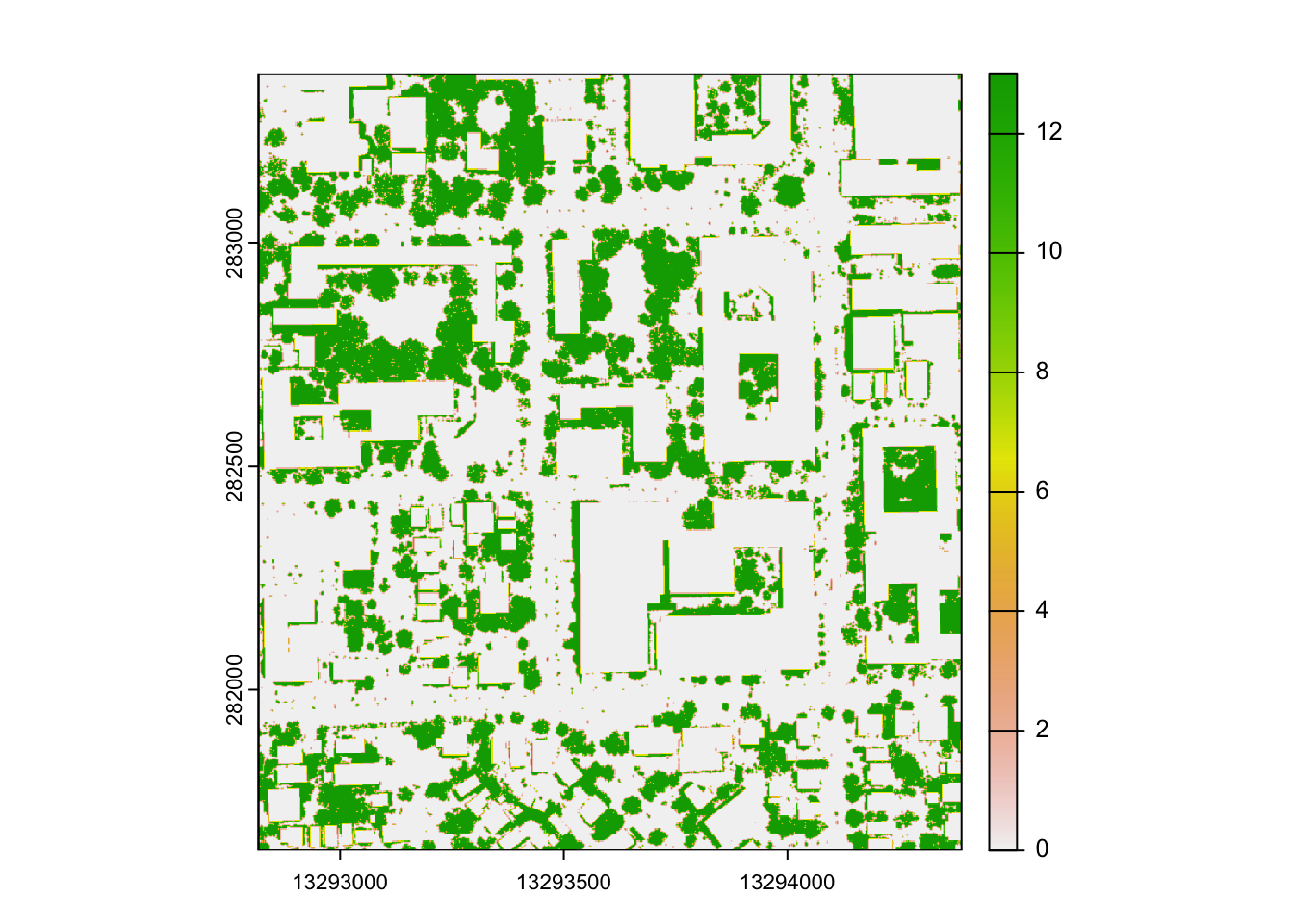
# read rasters of land use, canopy coverage, and building footprints
landuse <- terra::rast(system.file("test_landuse.tif",
package ="viewscape"))
canopy <- terra::rast(system.file("test_canopy.tif",
package ="viewscape"))
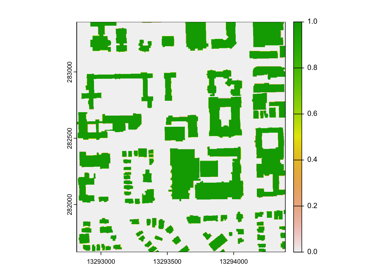
building <- terra::rast(system.file("test_building.tif",
package ="viewscape"))
terra::plot(dsm)
terra::plot(dtm)
terra::plot(landuse)
terra::plot(canopy)
terra::plot(building)
Second, I computed viewsheds for multiple viewpoints and specified parallel and workers in compute_viewshed().
# compute viewshed
viewsheds <- viewscape::compute_viewshed(dsm = dsm,
                                         viewpoints = viewpoints,
                                         offset_viewpoint = 6)
Third, I used functions, including calculate_diversity(), calculate_feature(), and calculate_viewmetrics(), to calculate:
- Shanon Diversity Index (SDI),
- depth,
- vdepth,
- extent,
- horizontal,
- relief,
- skyline,
- percentage of canopy and building,
- Number of patches (Nump),
- Mean shape index (MSI),
- Edge density (ED),
- Patch size (PS),
- Patch density (PD)
Let’s define a wrapped function. This has been saying that if one doesn’t have some layers, for example canopy and buildings
calculate <- function(viewsheds, dsm, dtm, land, canopy, building) {
  results <- matrix(0,length(viewsheds),16)
  colnames(results) <- c("x", "y", "Nump", "MSI", "ED", "PS", "PD",
                         "extent", "depth", "vdepth",
                         "horizontal", "relief", "skyline",
                         "sdi", "canopy", "building")
  masks <- list(canopy, building)
  for (i in 1:length(viewsheds)) {
    this_viewshed <- viewsheds[[i]]
    v_point <- this_viewshed@viewpoint
    metrics <- viewscape::calculate_viewmetrics(this_viewshed,
                                                dsm,
                                                dtm,
                                                masks = masks)
    results[i,1] <- v_point[1] # x
    results[i,2] <- v_point[2] # y
    results[i,3] <- metrics$Nump # Nump
    results[i,4] <- metrics$MSI # MSI
    results[i,5] <- metrics$ED # ED
    results[i,6] <- metrics$PS # PS
    results[i,7] <- metrics$PD # PD
    results[i,8] <- metrics$extent # extent
    results[i,9] <- metrics$depth # depth
    results[i,10] <- metrics$vdepth # vdepth
    results[i,11] <- metrics$horizontal # horizontal
    results[i,12] <- metrics$relief # relief
    results[i,13] <- metrics$skyline # skyline
    results[i,14] <- viewscape::calculate_diversity(this_viewshed, land) # sdi
    results[i,15] <- viewscape::calculate_feature(this_viewshed,
                                                  canopy, type = 2,
                                                  exclude_value = 0) # canopy
    results[i,16] <- viewscape::calculate_feature(this_viewshed,
                                                  building, type = 2,
                                                  exclude_value = 0) # building
  }
  return(results)
}
Now, run the function and check out the result.
result <- calculate(viewsheds, dsm, dtm, landuse, canopy, building)
head(result)
##             x        y Nump      MSI        ED        PS          PD extent
## [1,] 13294104 282359.0   47 2.650869 1.1041271  640.0387 0.007910045  63952
## [2,] 13293655 282911.7   20 2.794595 1.0541423  548.8783 0.007541369  28544
## [3,] 13293348 282548.5   66 2.839629 1.7903992  655.1316 0.010958980  64820
## [4,] 13293706 282004.4   75 3.504171 0.6253678  251.1605 0.012314330  65552
## [5,] 13293792 282431.5   12 2.013014 1.7917977 2543.1148 0.004046765  31916
## [6,] 13293971 283116.7   22 3.432804 1.4155829  717.2525 0.009962424  23768
##          depth    vdepth horizontal    relief  skyline   sdi    canopy
## [1,] 1018.8023 275.49927      48372 0.6656973 6.002534 0.790 0.2945334
## [2,]  446.5672  79.26814      17824 0.5784103 7.687110 0.128 0.3768217
## [3,]  748.8922 137.91273      38632 0.7132422 8.298789 0.733 0.2523295
## [4,]  889.6976 207.63062      52676 0.7954506 5.068768 0.947 0.1613986
## [5,]  843.2357 200.06310      26128 0.4780468 5.072695 0.693 0.2702093
## [6,]  445.0698 105.49972      14484 0.4915405 8.954859 1.160 0.3266577
##        building
## [1,] 0.10701776
## [2,] 0.07455157
## [3,] 0.27645788
## [4,] 0.08243837
## [5,] 0.06830430
## [6,] 0.22164254